203: Exampville Destination Choice¶

Welcome to Exampville, the best simulated town in this here part of the internet!

Exampville is a demonstration provided with Larch that walks through some of the data and tools that a transportation planner might use when building a travel model.

import larch.numba as lx
from larch import P, X

In this example notebook, we will walk through the estimation of a tour destination choice model. First, let’s load the data files from our example.

hh, pp, tour, skims, emp = lx.example(200, ['hh', 'pp', 'tour', 'skims', 'emp'])

For this destination choice model, we’ll want to use the mode choice logsums we calculated previously from the mode choice estimation, but we’ll use these values as fixed input data instead of a modeled value. We can load these logsums from the file in which they were saved. For this example, we can indentify that file using the larch.example function, which will automatically rebuild the file if it doesn’t exists. In typical applications, a user would generally just give the filename as a string and ensure manually that the file exists before loading it.

logsums_file = lx.example(202, output_file='logsums.zarr.zip')
logsums = lx.DataArray.from_zarr('logsums.zarr.zip')

Preprocessing¶

The alternatives in the destinations model are much more regular than in the mode choice model, as every observation will have a similar set of alternatives and the utility function for each of those alternatives will share a common functional form. We’ll leverage this by using idca format arrays in our DataTree to make data management simpler.

The base array we’ll start with will have two dimensions, cases and alternatives, anc be formed from the logsums we loaded above.

ca = lx.Dataset.construct(
    {'logsum': logsums},
    caseid='TOURID',
    alts=skims.TAZ_ID,
)
ca

<xarray.Dataset>
Dimensions:  (TAZ_ID: 40, TOURID: 7564)
Coordinates:
  * TAZ_ID   (TAZ_ID) int64 1 2 3 4 5 6 7 8 9 10 ... 32 33 34 35 36 37 38 39 40
  * TOURID   (TOURID) int64 0 1 3 7 10 13 ... 20728 20729 20731 20734 20736
Data variables:
    logsum   (TOURID, TAZ_ID) float64 dask.array<chunksize=(1891, 20), meta=np.ndarray>
Attributes:
    _caseid_:  TOURID
    _altid_:   TAZ_ID

For our destination choice model, we’ll also want to use employment data. This data, as included in our example, has unique values only by alternative and not by caseid, so there are only 40 unique rows. (This kind of structure is common for destination choice models.)

emp.info()

<class 'pandas.core.frame.DataFrame'>
Int64Index: 40 entries, 1 to 40
Data columns (total 3 columns):
 #   Column         Non-Null Count  Dtype
---  ------         --------------  -----
 0   NONRETAIL_EMP  40 non-null     int64
 1   RETAIL_EMP     40 non-null     int64
 2   TOTAL_EMP      40 non-null     int64
dtypes: int64(3)
memory usage: 1.2 KB

Then we bundle all our raw data into a DataTree structure, which is used to collect the right data for estimation. The Larch DataTree is a slightly augmented version of the regular sharrow.DataTree.

tree = lx.DataTree(
    base=ca,
    tour=tour.rename_axis(index='TOUR_ID'),
    hh=hh.set_index("HHID"),
    person=pp.set_index('PERSONID'),
    emp=emp,
    skims=lx.Dataset.construct.from_omx(skims),
    relationships=(
        "base.TAZ_ID @ emp.TAZ",
        "base.TOURID -> tour.TOUR_ID",
        "tour.HHID @ hh.HHID",
        "tour.PERSONID @ person.PERSONID",
        "hh.HOMETAZ @ skims.otaz",
        "base.TAZ_ID @ skims.dtaz"
    ),
)

Model Definition¶

Now we can define our choice model, using data from the tree as appropriate.

m = lx.Model(datatree=tree)
m.title = "Exampville Work Tour Destination Choice v1"

m.quantity_ca = (
        + P.EmpRetail_HighInc * X('RETAIL_EMP * (INCOME>50000)')
        + P.EmpNonRetail_HighInc * X('NONRETAIL_EMP') * X("INCOME>50000")
        + P.EmpRetail_LowInc * X('RETAIL_EMP') * X("INCOME<=50000")
        + P.EmpNonRetail_LowInc * X('NONRETAIL_EMP') * X("INCOME<=50000")
)

m.quantity_scale = P.Theta

m.utility_ca = (
    + P.logsum * X.logsum
    + P.distance * X.AUTO_DIST
)

m.choice_co_code = "tour.DTAZ"

m.lock_values(
    EmpRetail_HighInc=0,
    EmpRetail_LowInc=0,
)

Model Estimation¶

m.loglike()

-28238.336880999712

m.maximize_loglike()

Iteration 013 [Optimization terminated successfully]

Best LL = -25157.723517429302

	value	initvalue	nullvalue	minimum	maximum	holdfast	best
EmpNonRetail_HighInc	1.363964	0.0	0.0	-inf	inf	0	1.363964
EmpNonRetail_LowInc	-0.881402	0.0	0.0	-inf	inf	0	-0.881402
EmpRetail_HighInc	0.000000	0.0	0.0	0.000	0.0	1	0.000000
EmpRetail_LowInc	0.000000	0.0	0.0	0.000	0.0	1	0.000000
Theta	0.749368	1.0	1.0	0.001	1.0	0	0.749368
distance	-0.041820	0.0	0.0	-inf	inf	0	-0.041820
logsum	1.020788	0.0	0.0	-inf	inf	0	1.020788

/home/runner/work/larch/larch/larch/larch/model/optimization.py:308: UserWarning: slsqp may not play nicely with unbounded parameters
if you get poor results, consider setting global bounds with model.set_cap()
  warnings.warn( # infinite bounds # )

key

value

x

	0
EmpNonRetail_HighInc	1.363964
EmpNonRetail_LowInc	-0.881402
EmpRetail_HighInc	0.000000
EmpRetail_LowInc	0.000000
Theta	0.749368
distance	-0.041820
logsum	1.020788

loglike

-25157.723517429302

d_loglike

	0
EmpNonRetail_HighInc	0.000563
EmpNonRetail_LowInc	0.004877
EmpRetail_HighInc	0.000000
EmpRetail_LowInc	0.000000
Theta	0.004725
distance	-0.063393
logsum	0.021062

nit

13

nfev

32

njev

13

status

0

message

'Optimization terminated successfully'

success

True

elapsed_time

0:00:01.530184

method

'slsqp'

n_cases

7564

iteration_number

13

logloss

3.3259814274761106

m.calculate_parameter_covariance()

Model Visualization¶

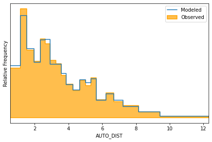
For destination choice and similar type models, it might be beneficial to review the observed and modeled choices, and the relative distribution of these choices across different factors. For example, we would probably want to see the distribution of travel distance. The Model object includes a built-in method to create this kind of visualization.

m.distribution_on_idca_variable('AUTO_DIST')

<AxesSubplot:xlabel='AUTO_DIST', ylabel='Relative Frequency'>

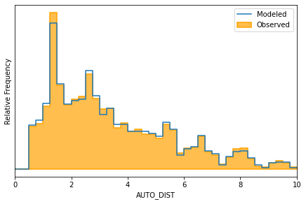
The distribution_on_idca_variable has a variety of options, for example to control the number and range of the histogram bins:

m.distribution_on_idca_variable('AUTO_DIST', bins=40, range=(0,10))

<AxesSubplot:xlabel='AUTO_DIST', ylabel='Relative Frequency'>

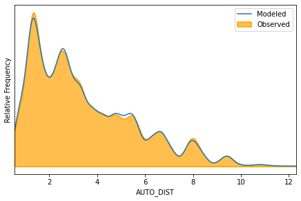
Alternatively, the histogram style can be swapped out for a smoothed kernel density function:

m.distribution_on_idca_variable(
    'AUTO_DIST',
    style='kde',
)

<AxesSubplot:xlabel='AUTO_DIST', ylabel='Relative Frequency'>

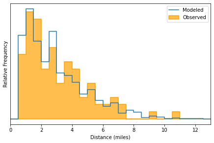
Subsets of the observations can be pulled out, to observe the distribution conditional on other idco factors, like income.

m.distribution_on_idca_variable(
    'AUTO_DIST',
    xlabel="Distance (miles)",
    bins=26,
    subselector='INCOME<10000',
    range=(0,13),
    header='Destination Distance, Very Low Income (<$10k) Households',
)

<AxesSubplot:xlabel='Distance (miles)', ylabel='Relative Frequency'>

Save and Report Model¶

report = lx.Reporter(title=m.title)

report << '# Parameter Summary' << m.parameter_summary()

Parameter Summary

	Value	Std Err	t Stat	Signif	Null Value	Constrained
EmpNonRetail_HighInc	1.36	0.256	5.32	***	0.00
EmpNonRetail_LowInc	-0.881	0.0791	-11.14	***	0.00
EmpRetail_HighInc	0.00	NA	NA		0.00	fixed value
EmpRetail_LowInc	0.00	NA	NA		0.00	fixed value
Theta	0.749	0.0152	-16.45	***	1.00
distance	-0.0418	0.0107	-3.90	***	0.00
logsum	1.02	0.0317	32.16	***	0.00

report << "# Estimation Statistics" << m.estimation_statistics()

Estimation Statistics

Statistic	Aggregate	Per Case
Number of Cases	7564
Log Likelihood at Convergence	-25157.72	-3.33
Log Likelihood at Null Parameters	-28238.34	-3.73
Rho Squared w.r.t. Null Parameters	0.109

report << "# Utility Functions" << m.utility_functions()

Utility Functions

+ P.logsum * X.logsum
+ P.distance * X.AUTO_DIST
+ P.Theta * log(
   + exp(P.EmpRetail_HighInc) * X('RETAIL_EMP * (INCOME>50000)')
   + exp(P.EmpNonRetail_HighInc) * X('NONRETAIL_EMP*(INCOME>50000)')
   + exp(P.EmpRetail_LowInc) * X('RETAIL_EMP*(INCOME<=50000)')
   + exp(P.EmpNonRetail_LowInc) * X('NONRETAIL_EMP*(INCOME<=50000)')
)

The figures shown above can also be inserted directly into reports.

figure = m.distribution_on_idca_variable(
    'AUTO_DIST', 
    xlabel="Distance (miles)",
    style='kde',
    header='Destination Distance',
)
report << "# Visualization"
report << figure

Visualization

report.save(
    'exampville_dest_choice.html',
    overwrite=True,
    metadata=m,
)

'exampville_dest_choice.html'

v5.7.0

203: Exampville Destination Choice

Contents